Finding the optimal charging station stop with Kinetica
You are in an electric car that is almost out of charge. There are several charging stations that you can stop at. Which one should you pick en route to your destination?
In this demo, we use Kinetica’s graph API to create a 1.2 million node graph representation of the road network in and around Detroit. We then use this graph network to find the optimal route between a source and destination point by picking the best charging station out of 268 different options. We repeat these computations every 5 seconds using a SQL procedure with new sets of source and destination points that are streaming in from a Kafka topic.
There are three steps in this analysis.
- Find the shortest path from source point to all the charging stations that are within range (i.e. before the car runs out of charge).
CREATE OR REPLACE TABLE ev_route_optimization.source_to_charging_path AS
    SELECT *
    FROM TABLE (
        SOLVE_GRAPH
        (
            GRAPH => 'ev_route_optimization.mm_lakes',
            SOLVER_TYPE => 'SHORTEST_PATH',
            SOURCE_NODES => INPUT_TABLE(
                SELECT ST_GEOMFROMTEXT(source_pt) AS WKTPOINT
                FROM ev_route_optimization.source_dest
                ORDER BY TIMESTAMP DESC -- Find the latest source record
                LIMIT 1
            ),
            DESTINATION_NODES => INPUT_TABLE(
                SELECT
                    Longitude AS X,
                    Latitude AS Y
                FROM ev_route_optimization.mm_evcharging
            ),
            OPTIONS => KV_PAIRS(max_solution_radius = '2400')
        )
    );
- Compute the inverse shortest path from all the charging stations to the destination.
    CREATE OR REPLACE TABLE ev_route_optimization.charging_to_dest_path AS
    SELECT *
    FROM TABLE (
        SOLVE_GRAPH
        (
            GRAPH => 'ev_route_optimization.mm_lakes',
            SOLVER_TYPE => 'INVERSE_SHORTEST_PATH',
            SOURCE_NODES => INPUT_TABLE(
                SELECT ST_GEOMFROMTEXT(dest_pt) AS WKTPOINT
                FROM ev_route_optimization.source_dest
                ORDER BY TIMESTAMP DESC -- Find the latest destination record
                LIMIT 1
            ),
            DESTINATION_NODES => INPUT_TABLE(
                SELECT
                    Longitude AS X,
                    Latitude AS Y
                FROM ev_route_optimization.mm_evcharging
            )
        )
    );
- Combine the two to find the optimal path with the lowest total cost.
INSERT INTO ev_route_optimization.optimal_route /* ki_hint_update_on_existing_pk */
    SELECT *
    FROM
    (
        WITH temp (id_with_min_cost) AS
        (
            SELECT arg_min(s1+s2,id1) as id_with_min_cost FROM
                (SELECT  SOLVERS_NODE_COSTS as s1, SOLVERS_NODE_ID as id1, * from ev_route_optimization.source_to_charging_path),
                (SELECT  SOLVERS_NODE_COSTS as s2, SOLVERS_NODE_ID as id2, * from ev_route_optimization.charging_to_dest_path)
            WHERE id1 = id2
        )
        SELECT
            1 as pk_id,     --this is the primary key so we will always be overwriting this record
            s1.wktroute as wkt1,
            s2.wktroute as wkt2,
            st_linemerge(st_collect(s1.wktroute,s2.wktroute)) as wkt_full
        FROM
            ev_route_optimization.source_to_charging_path s1,
            ev_route_optimization.charging_to_dest_path s2,
            temp
        WHERE
            s1.SOLVERS_NODE_ID = temp.id_with_min_cost and
            s2.SOLVERS_NODE_ID = temp.id_with_min_cost
    );
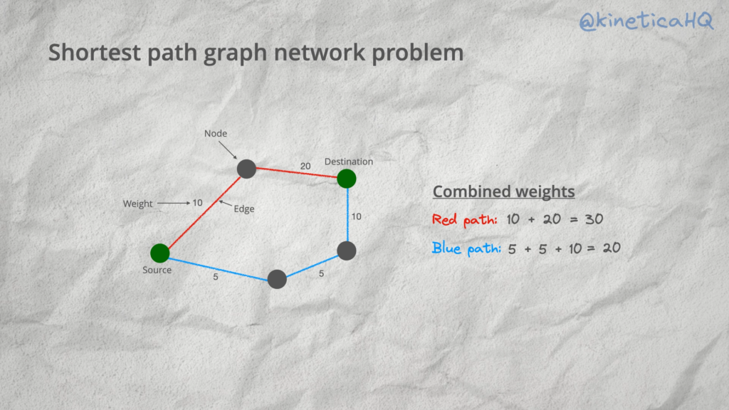
Shortest path solvers are used to find the optimal path between two points on a graph network that has the lowest combined edge weights. Edge weights can be used to optimize for things like distance, the time taken or even something random like say how scenic a route is. We can pretty much model anything as long as we have data on it.
The entire analysis is done with SQL on a small instance of Kinetica on Azure. We have set up all the data so that the example is fully reproducible. Follow the instructions below to try this out on your own.
Try it yourself
All you need to get started is an instance of Kinetica and the workbook file.
The workbook file is available here.
Kinetica is available via Azure and AWS as a managed service, it can also be installed and run on your local machine as a Docker container. Follow the instructions here to install Kinetica.
If you have any questions, you can reach us on Slack and we will get back to you immediately.
Watch the demo
Making Sense of Sensor Data