Window functions allow us to perform calculations on a subset of rows in a table, rather than the entire table.
A window function performs a calculation across a set of rows that are related to the current row, based on a specified window of observations. They are used to calculate running totals, ranks, percentiles and other aggregate calculations that can help identify patterns or trends within groups. Let's look at how to use window functions in SQL.
The code below shows a moving average calculation that uses a window function. It applies the average function over a window with five observations that is partitioned by a stocks symbol and ordered by time.
AVG(price_close) OVER (
    PARTITION BY symbol
    ORDER BY time
    ROWS 5 PRECEDING
) AS avg_price
Let's break this down to understand the purpose of each of these clauses.
Apply Function OVER a Window
At the most abstract level, we can think of a window function as being applied on a "window" of rows that are related to the current row. The specified window slides with the "current row" so that the set of values that a window function is applied to updates with each row (see animation below). The window function generates one result value per row thereby allowing us to preserve the original granularity of the data.
The window function above calculates the rolling average price for the past five observations using a window for the AAPL (Apple) stock price.
This is a simple illustration of a window function. It works because the rows in the table are ordered by the time column and because the only stock symbol is AAPL so the previous five rows correspond to the last five observations of AAPL.
But what if the rows in the table were not ordered by the timestamp? Or if there were other stock
symbols in the table. These cases are handled using the
ORDER BY
and
PARTITION BY
clauses in the window function. Let's explore these next.
ORDER BY
The animation below illustrates the
ORDER BY
clause. The table is initially not ordered by the timestamp column. As a result, the average is not
being computed on the previous five observations. We can fix this by simply ordering the data on the
time column. Note that the window function does not update the actual ordering of the table itself, it
simply reorders the rows for the sake of performing the calculation without mutating the table itself.
This is important since it doesn't inadvertently affect other queries that might require the table to
be ordered on a column other than time.
Now, let's introduce another layer of complexity. Imagine that the table includes two additional stock symbols — GOOG (Google) and AMZN (Amazon).
PARTITION BY
We can address this by partitioning the data on the stock symbol column.
By partitioning the data by each stock, we apply the window on observations within each partition rather than across them. Note that just like the ordering clause, partitioning the table does not replace the structure of the input table.
The final piece in a window function is the sizing of the window itself — the "frame."
Framing a Window
So far, we have positioned the window above the current row with an arbitrary number of rows as its size. But what if we wanted to position the window elsewhere (above the current row, including the current row, from start, etc.)? The frame clause inside a window specification offers a great deal more flexibility and control over the sizing of a window.
There are two types of frame clauses, rows and range. A range clause considers the values of the records in the ordering column. While a row clause considers the ordering of the records. This can be a bit hard to understand when written down but the distinction between the two crystallizes when we encounter duplicate (or "peer") values in the ordering column.
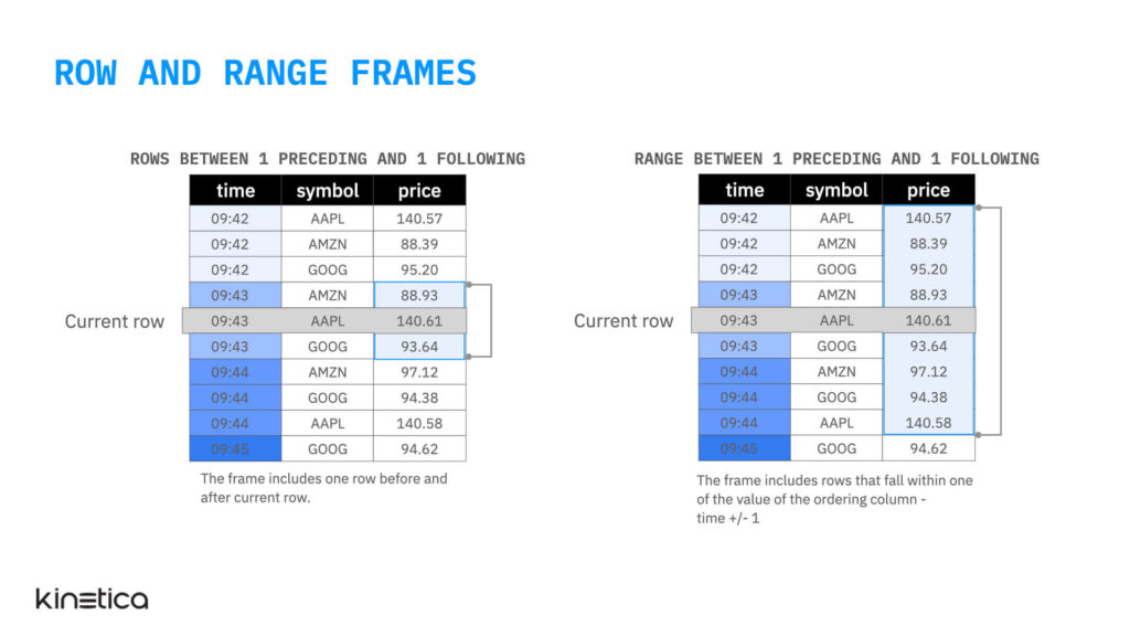
The tables in the illustration below have duplicate values in the ordering column time. Let's ignore the partitioning for now. A row clause that specifies a frame with one row preceding and following the row will result in a frame with three observations in it — the row preceding the current row, the current row and the row following the current row. The range clause on the other hand yields a window that has nine rows in it — all the records with value of time (the ordering column) that fall within a range one less than or one more than the time of the current row. This includes all records with a time in the range 9:42 to 9:44
There are a few options when setting the start and end points for a frame. These are listed below along with their description.
Frame start keywords |
UNBOUNDED PRECEDING | The first row of the partition |
| <number> PRECEDING | Either n rows before the current row (for rows-based frames) or n values less than the current row's value (for range-based frames) | |
| CURRENT ROW | Either the current row (for rows-based frames) or the current row and its peer rows (for range-based frames) | |
| <number> FOLLOWING | Either n rows after the current row (for rows-based frames) or n values greater than the current row's value (for range-based frames) | |
Frame end keywords |
UNBOUNDED FOLLOWING | The last row of the partition |
| <number> FOLLOWING | Either n rows after the current row (for rows-based frames) or n values greater than the current row's value (for range-based frames) | |
| CURRENT ROW | Either the current row (for rows-based frames) or the current row and its peer rows (for range-based frames) | |
| <number> PRECEDING | Either n rows before the current row (for rows-based frames) or n values less than the current row's value (for range-based frames) |
Now, let's check out a few examples for common window function queries.
A Moving Average with Row-Based Frames
The query below is an illustration of a simple moving average. The partition by clause separates the rows based on the stock symbol, the ordering clause arranges the rows within each stock partition in descending order of time, and the row clause specifies a window frame with five observations before the current row.
SELECT
    time,
    symbol,
    AVG(price_close) OVER
        (
            PARTITION BY symbol
            ORDER BY time
            ROWS 5 PRECEDING
        ) AS mov_avg_price
FROM trades
A Moving Average with Range-Based Frames
The query below is similar to the one above but with one important difference. We are using a range-based frame instead of a row. The range clause specifies a frame with all observations that have a time value within five minutes (300,000 milliseconds) of the current row. This includes observations before and after the current row.
SELECT
    time,
    symbol,
    AVG(price_close) OVER
        (
            PARTITION BY symbol
            ORDER BY time
            RANGE BETWEEN 300000 PRECEDING AND 300000 FOLLOWING
        ) AS mov_avg_price
FROM trades
Ranking
So far we have seen aggregate functions that summarize the observations in a particular window frame. Ranking functions comprise another type of window functions. They are used to compare data points within a given series or between different series and determine their relative importance. In the query below, I am using a ranking function to rank the closing prices of different stocks. Notice how the ordering column is now the closing price and not time. This is because the rank is determined based on the ordering column.
SELECT symbol, time price_close,
    RANK() OVER (
       PARTITION BY symbol
       ORDER BY price_close DESC
    ) AS high_price_rank
FROM trades
ORDER BY high_price_rank
Try This on Your Own
Kinetica offers 18 different window functions (aggregate + ranking). And the time series workbook contains several window functions and it is a good starting point.
You can import this workbook into Kinetica Cloud or Kinetica's Developer Edition to try these out on your own. I have pre-configured all the data streams so you don't have to do any additional setup to run this workbook.
Both Kinetica Cloud and Developer Edition are free to use. The cloud version takes only a few minutes to set up and it is a great option for quickly touring the capabilities of Kinetica. The Developer Edition is also easy to set up and takes about 10 to 15 minutes and an installation of Docker. The Developer Edition is a free forever personal copy that runs on your computer and can handle real-time computations on high-volume data feeds.