B. Kaan Karamete, PhD, is Senior Director of Engineering for Geospatial, Graph, and Visualization at Kinetica
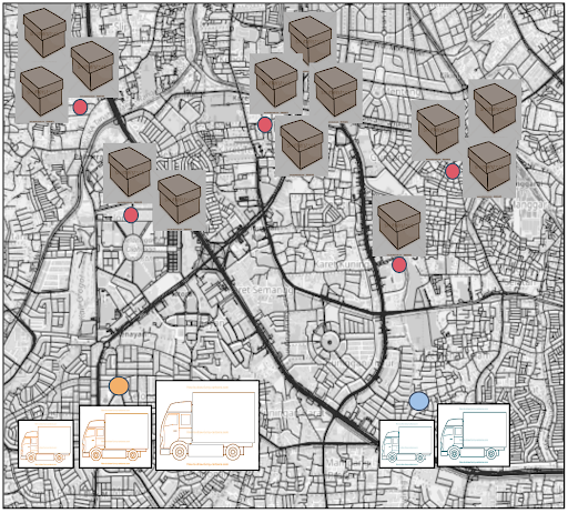
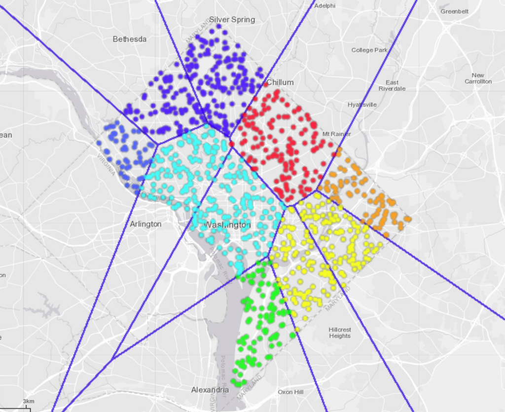
Matching supply chain logistics to demand based routing is a daily, non-trivial task essential to several companies like Amazon and Uber. The common objective is to optimize routing under domain specific constraints to the needs of a particular industry. We developed our own Multiple Supply Demand Chain Optimization (MSDO) graph solver in order to provide a generic and uniformly applicable solution to the needs of different industries. The optimization quantity could be the power transported by the transformers to multiple consumers with different power needs, or tons of gasoline transported by tankers to various stations, or simply the packets of goods delivered from multiple depots to multiple geographical locations. The main point in all of these transport problems is that neither the supply, nor the demand side transport quantity is a constant. For instance, a depot can have many vehicles with a variety of truck capacities to deliver varying amounts of goods at each customer location spread across a vast geography as seen below. The ultimate goal is to find the ‘optimal’ routing and scheduling for each truck individually such that the total transportation cost is minimized. The ‘optimality’ criterion could be the minimization of the total cost either in terms of the distance travelled by all the trucks (transport vehicles) subject to the underlying road network’s speed and turn restrictions/penalties or the total time subject to the delivery priorities. Whatever the optimality criterion and multiple constraints are, mathematically speaking, the task is simply the minimization of the overall transport cost subject to multiple constraints defined over a network graph.
Kinetica Graph is designed and implemented from scratch and built over a set of network agnostic graph grammar. The key differentiator of Kinetica Graph DB from its competitors is its efficient data representation supporting a very large number of edges/nodes that has no memory degradation under dynamic updates. Our optimized parallel Graph Solvers are built on top of this representation. Kinetica Graph also works in tandem with the distributed relational Kinetica DB for I/O, and seamlessly integrates at-scale OLAP expression support with hundreds of PostGIS geometry functions.
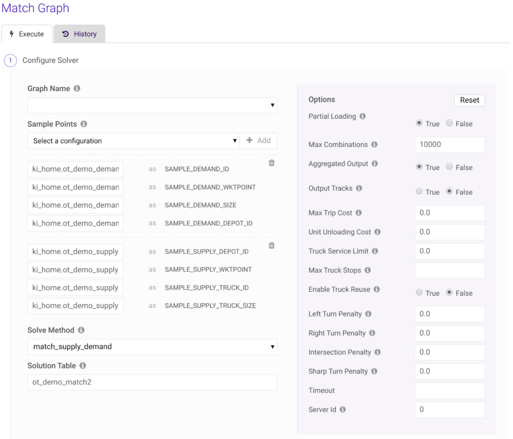
Real time multiple supply demand chain optimization routing solver (MSDO) algorithm enumerates millions of combinations in milliseconds and provides the dynamic routing and tracking capability for the entire distribution fleet to thousands of customer locations in the most optimal manner. MSDO solver’s optimization engine honors multiple constraints in terms of the maximum thresholds on truck operation limits, maximum distance between consecutive stops, unit unloading time, and customer priorities. The optimization algorithm ensures the most optimal routing without blending these constraints, but rather satisfying them while processing all (reasonable) combinations. Additional constraints of truck reuse and turn restrictions/penalties are also taken into account. MSDO solver is supported by our /match/graph endpoint by a simple to use, server side, RESTFUL schema available in SQL, R, Python, C++, Java and JavaScript language APIs. An intuitive Graph-UI is also envisaged within our Kinetica-GAdmin application to provide ease of use to our clients as shown on the side. MSDO solver outputs the results to a Kinetica DB table as shown below.
Optionally, the output can also be converted to tracks with correct timestamps, to be consumed by our /create/video endpoint for enabling real-time dynamic routing simulations. Similarly, truck paths can be visualized using our distributed rendering capabilities via an WMS request as shown below.
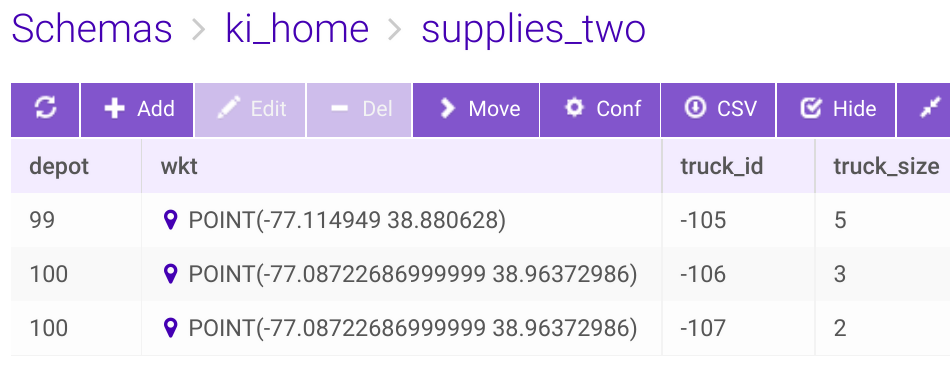
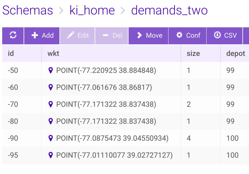
A simple MSDO test scenarioX can be demonstrated here with two depots in Table supplies_two that has three trucks in different capacities, and another Table demands_two with six customer locations (two with an identical lon/lat address), and each with varying number of demands, respectively, as shown below.
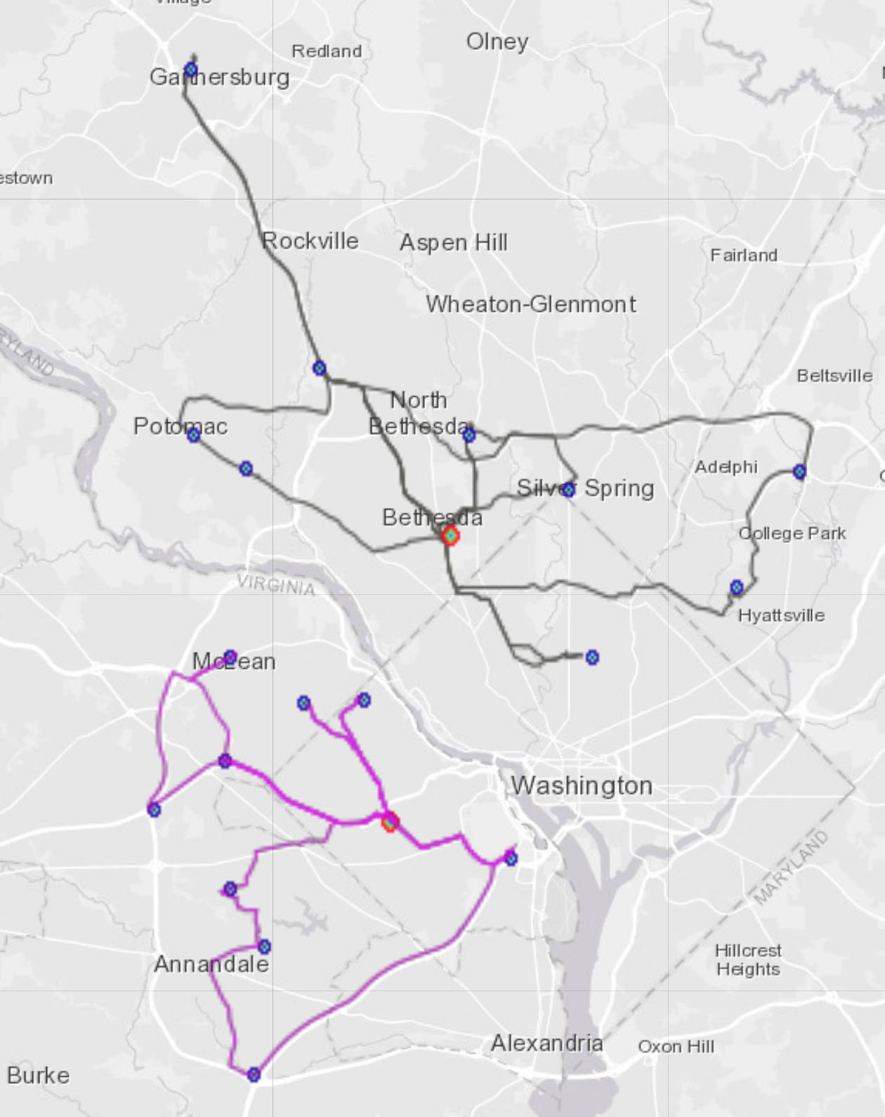
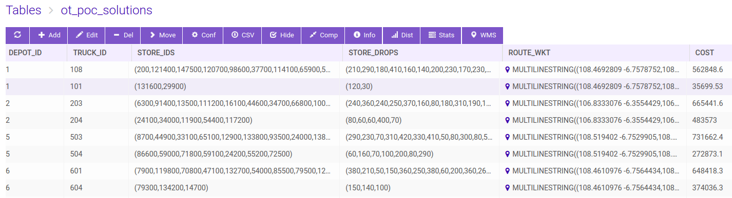
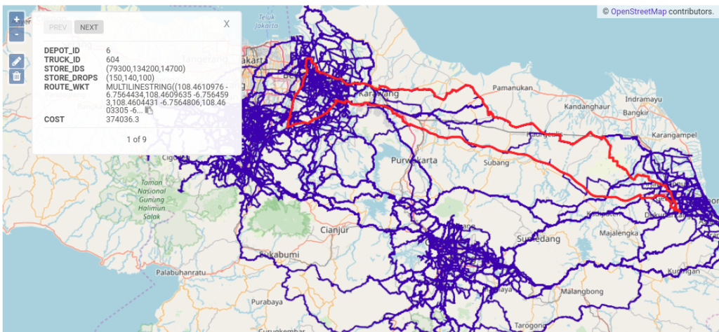
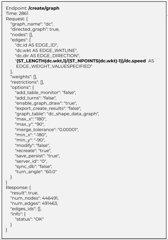
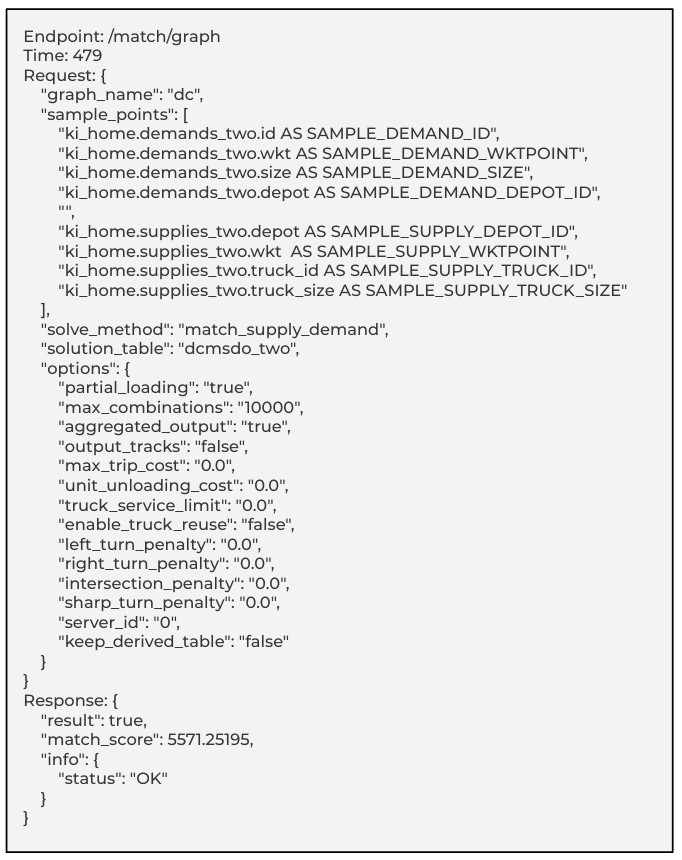
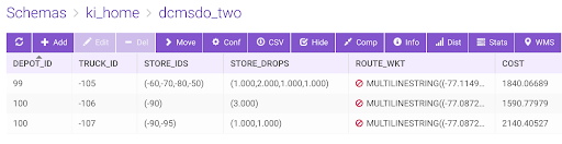
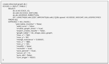
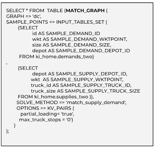
The DC road network graph is created via the /create/graph endpoint with edge weights in time calculated by an OLAP expression that takes into account the geodesic length of the road segments and the permitted speed limits. We can then solve on this directed DC graph by invoking our /match/graph endpoint with the solve_method set to ‘match_supply_demand’. Having set the supply and demand component combination parameters, essentially mapping the input table columns with our graph grammar, we get the optimal routing results in milliseconds. The output table has the routing results per truck on each record row with aggregated drop list, and demand locations as well as the MULTILINESTRING WKT road path due to the ‘aggregated_output’ option. We can also visually inspect these routes by clicking on the WMS button of the table UI which spawns another Kinetica endpoint that renders the WKT paths in a distributed manner where the image in the viewport is constructed from the partial PNGs generated at each worker rank concurrently. Endpoint calls and output can be seen below.
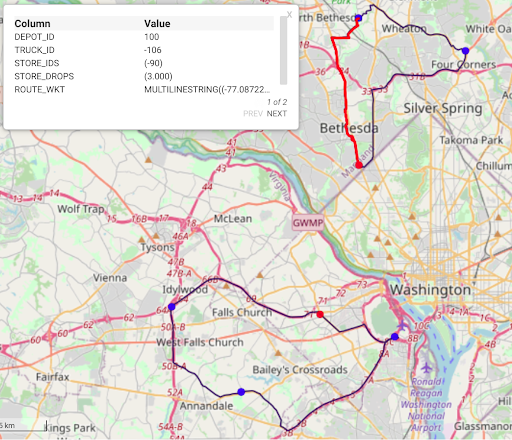
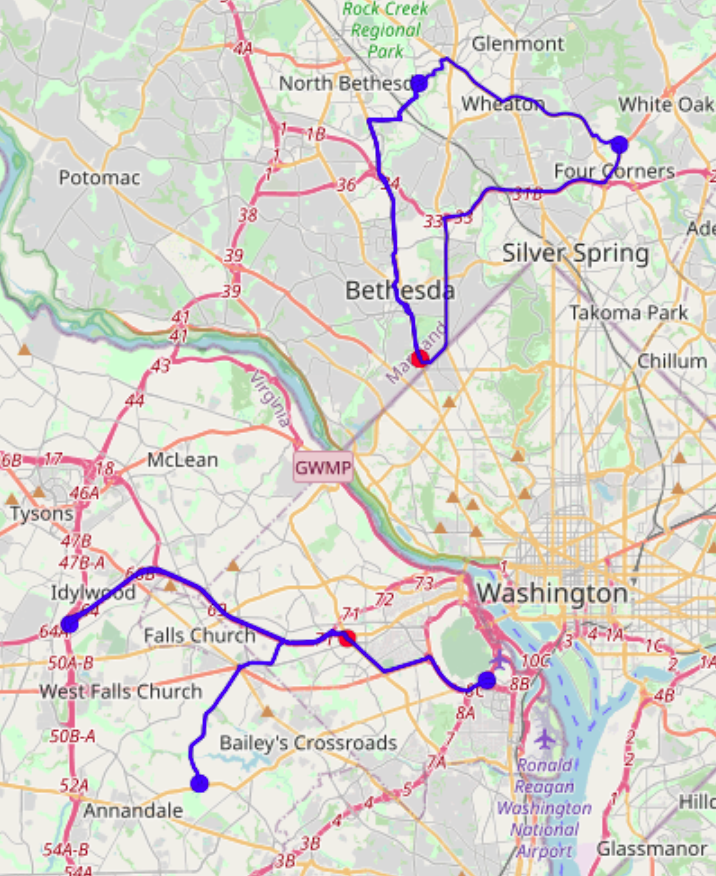
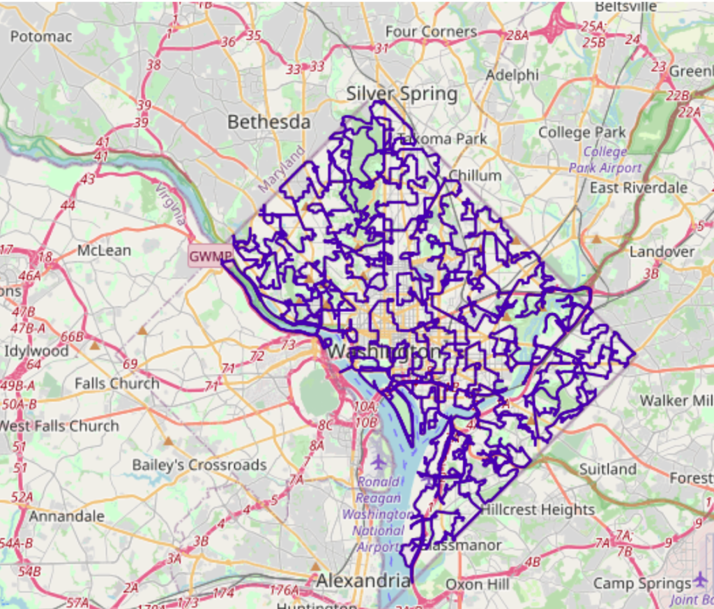
The WMS output is showing all of the truck routes originating from their respective depots, and dropping off at customer locations either the whole or partial amounts depending on the ‘partial_loading’ option. The route shown by the red path in the picture denotes the path for truck -106 which drops at demand side -90 all of its capacity of 3 units and returns back to its depot. If we’d like to run a different scenario with a constraint of allowing maximum of two customers to be visited by the same truck, then truck -105 would not be able to deliver to all four locations and since total demand is exactly equal to the total supply, the only way then to make the supply matching the demand would have been to allow the option ‘enable_truck_reuse’. Rerunning the /match/graph with these new options, gives two round-trip paths for the truck -105, which can be seen in the output table and the image below.
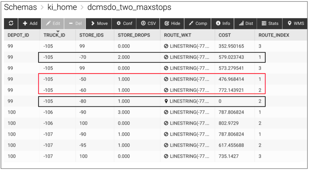
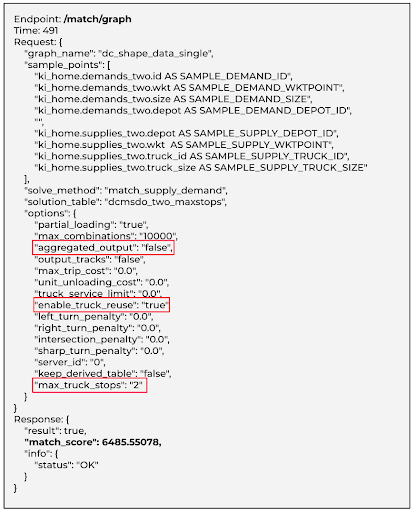
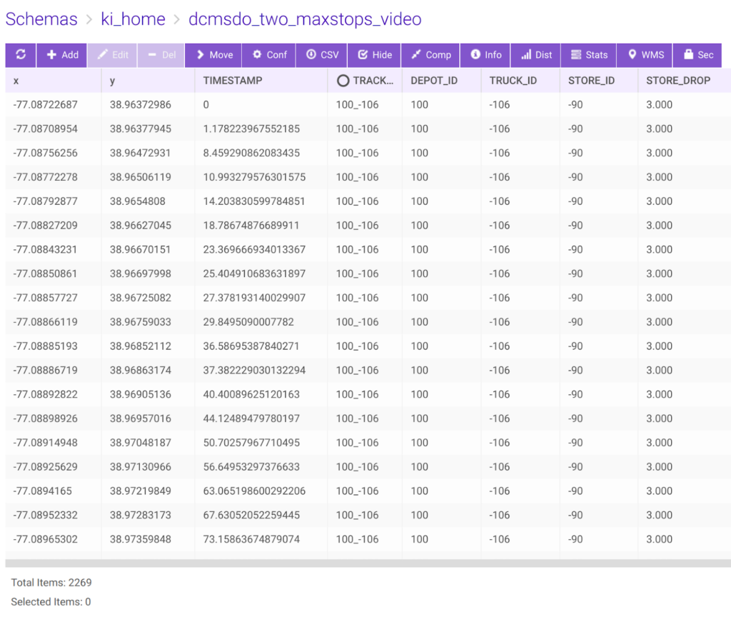
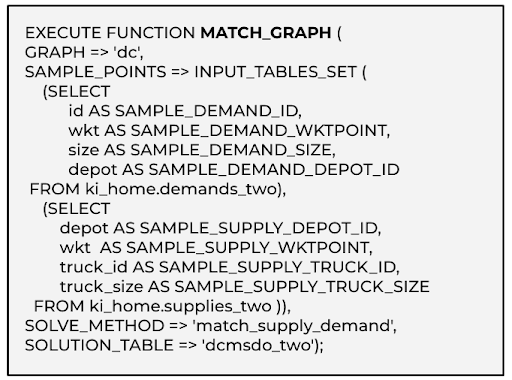
It is worth noting that the output table format is an unpivoted one, i.e., ‘aggregated_output’ is false, hence each record row gives only one leg of the trip, with its ‘ROUTE_INDEX’ column depicting its order index in the round trip. As expected, the total cost of the match is increased due to the ‘max_truck_stops’ constraint.. Furthermore, a video output can also be generated from the MSDO output which translates the paths into time-stamped tracks accurately set by the weights of the graph, giving the ability to simulate the entire fleet scheduling with real time values. This enables us to track the movement of each truck, and makes it possible to alert higher level applications for oversight and to make necessary adjustments to account for any deviations from the scheduled deliveries. The same create/graph and match/graph APIs can easily be run via our Integrated Analytics SQL engine below:

Finally, MSDO is an at-scale and at-pace solver, in the sense that the graph can be replicated/distributed over many nodes (ranks), thereby partitioning the requested task and running the scheduler on multi- threads of each rank which makes it a truly parallel solver. We have recently demonstrated MSDO to a retailer company operating in greater Jakarta region, using the data from their day-to-day operations, as a proof of concept involving the scheduling of 1,000 trucks over 72 depots delivering to 3,500 customers in less than two minutes on a single node of a 540 GByte, 80 core machine over the entire road network graph of greater Jakarta region shown in the Table ot_poc_solution and WMS image on Page 2 above.
Another problem case is a classic multiple travelling salesman problem: One thousand random locations are generated and depicted as collection locations within the metropolitan region of Washington-DC. Kinetica’s ST_voronoi geometry function is invoked followed by a geo-join operation to split and assign 1000 collections to 10 collectors (generator points in Voronoi partitioning are user-prescribed). The problem is to find the optimal round trips for each of these ten collectors. This classic multiple Travelling salesman problem can be cast into MSDO format as if there is one truck at each collector of size equal to the number of collections they each need to visit. Each collection should exactly have a demand size of one unit. The video generated from the tracks output of MSDO can be seen below:

(x) For the two depot MSDO example case demonstrated in this blog download the data set msdo.tar.gz