Real-time location intelligence is the the art of gathering, analyzing and acting on location-based data as events unfold. It’s valuable for a range of applications such as fleet management, smart cities, detecting threats in our airspace, smart agriculture, proximity marketing, telco network optimization, supply chain management and more.
Over the past few years, building real-time location intelligence solutions has become easier thanks to the introduction of new specialized technologies that are designed to handle the processing, analysis and visualization of location-based data.
In this article, you will learn how to set up a location intelligence pipeline that is built on top of real-time data feeds from Apache Kafka. The workbook contains an end-to-end pipeline that connects to streaming data sources via Kafka, performs spatial computations to detect different events and patterns, and then streams these to an external application. All of this is done using simple SQL code without any need for complicated data engineering. You can follow along using the Kinetica workbook in this link.
Setup
There are a few things to consider when picking a database for real-time spatial analysis.
- Native connectors to streaming data sources like Kafka
- Functional coverage: The ST_Geometry library from PostGIS is the gold standard for geospatial functions. Most spatial databases emulate this library.
- Spatial joins: The ability to combine multiple tables based on a spatial relationship. This is important for any type of sophisticated analysis of spatial data.
- Performance: Real-time applications require spatial functions to be executed on large amounts of data at high speeds.
- Reactivity: The system needs to automatically detect and respond to new data without any elaborate engineering on our part.
- Integrated capabilities: Location intelligence workloads often have niche analytical requirements such as routing and optimization using graph networks and the ability to visualize large amounts of data.
- Stream data out: The final piece of the pipeline is the ability to stream data out of an analytical database into external systems.
This demo uses Kinetica’s free developer edition to run the queries in this article. See the last section of this article for more information on how to try the queries here on your own.
Data
We will use the following data for this demo.
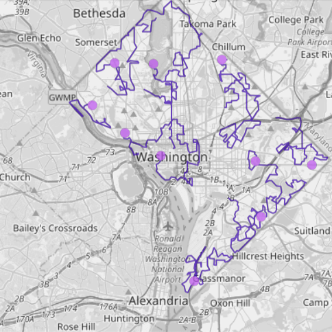
- A stream of GPS coordinates that record the movement of seven trucks in Washington, D.C. The data is being streamed in via a Kafka topic.
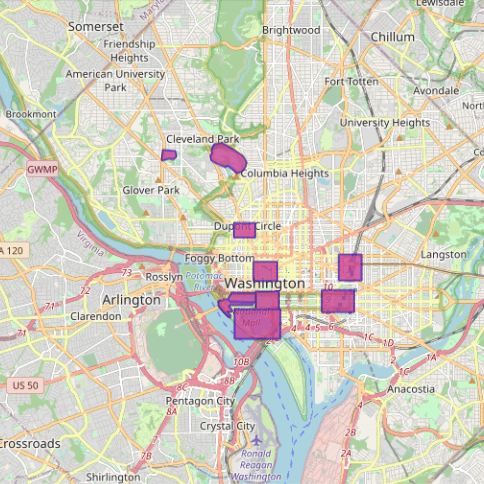
- A set of polygons that outline different landmarks in D.C.
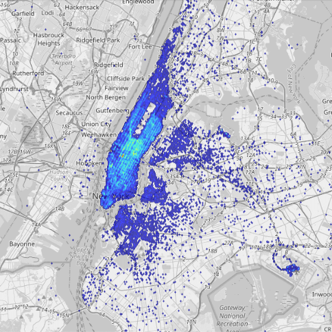
- A stream of taxi trips that are occurring in New York City (a few hundred per second)
All the data feeds are preconfigured so you don’t have to do any setup to replicate the queries here on your own. The maps below are a visual representation of the data.
Let’s dive into a few common analytical tasks that underpin location intelligence.
Spatial Filtering
A spatial filter is used to identify a subset of records from a table that meet some criteria based on a specific spatial query.
Let’s start with a really simple query to kick things off. The query below, identifies all the “fences” — the outlines around landmarks that have an area greater than 0.5 km2 (500,000 m2).
CREATE OR REPLACE TABLE fence_filter AS
SELECT wkt
FROM dc_fences
WHERE ST_AREA(wkt, 1) > 500000
This is a pretty easy query to implement in any database that supports spatial operations since it is filtering from a small table. Now let’s explore a few use cases that are harder to implement in real time.
Spatial Join of Streaming Locations with the Fences Table
Spatial joins combine two different tables using a spatial relationship. They are used to answer questions such as “which areas overlap,” “where do the boundaries occur” and “what is the area covered by a certain feature.” Spatial joins are typically computationally expensive to perform, especially on larger data.
The query below performs an inner join between the recent_locations table and the dc_fences table that outlines landmarks in D.C. based on the following criteria: Find all records where a truck came within 200 meters of a landmark in D.C.
CREATE OR REPLACE MATERIALIZED VIEW vehicle_fence_join
REFRESH ON CHANGE AS
SELECT
    TRACKID,
    x,
    y,
    DECIMAL(STXY_DISTANCE(x, y, wkt, 1)) AS distance,
    fence_label,
    wkt
FROM recent_locations
INNER JOIN dc_fences
    ON
    STXY_DWITHIN(x, y, wkt, 200, 1) = 1;
Everything looks similar to PostGIS but …
This query looks remarkably similar to any query that you might see in PostGIS or any other spatial database that uses ST_Geometry. The key difference, however, is the use of the materialized view that is set to refresh on change. This means that the query will be updated in real time as new records with truck location hit the Kafka topic.
With this change, the database will constantly monitor and maintain the join view (vehicle_fence_join) to reflect the most up-to-date version of truck locations. Or in other words, if there is a new truck location that is close to a landmark, it will be automatically reflected in the join view.
Take It up a Notch with a Time Filter
In the previous query we identified all the records that matched spatial criteria. Now, let’s add time-based criteria.
The query below identifies all instances from the last 5 minutes where a truck location was inside one of the “fences” around a landmark in Washington, D.C.
CREATE OR REPLACE MATERIALIZED VIEW fence_events
REFRESH ON CHANGE AS
SELECT
    TRACKID,
    wkt,
    x,
    y,
    TIMESTAMP,
    CONCAT(TRACKID, CONCAT(' is at ', fence_label)) AS event_text
FROM recent_locations, dc_fences
WHERE
    STXY_CONTAINS(wkt, x, y) = 1 AND
    TIMEBOUNDARYDIFF('MINUTE', TIMESTAMP, NOW()) < 5
The query above performs a very common location intelligence task: geofencing. Geofencing is a location-based service in which a software application uses GPS, RFID, Wi-Fi or cellular data to trigger a preprogrammed action when an object enters or exits a virtual boundary set up around a geographical location. Geofencing can be used for various purposes, such as sending notifications to customers when they enter or leave an area, providing targeted advertising based on location, and tracking employee time and attendance.
Now, there is one particular scenario where the query we used above will fail. Consider a fence that is really small; an object might enter this fence and then subsequently exit before it emits a location signal. Or in other words, if we don’t have data on a geofence event, we won’t be able to detect it.
But there is a workaround for this. We can interpolate the “track” between two subsequent points to then infer if the track intersects with the fence. Let’s look at that next.
Add Interpolation with Tracks for More Accurate Detection
The animation below shows the scenario we just described. Without interpolation it might seem that a particular object did not enter a fence. But with interpolation, we can correctly infer that the track did indeed intersect with a fence.
Kinetica offers a native track object that does all the interpolation behind the scenes. A track requires the following information: a timestamp (so that we know the order of the points), the X and Y (longitude/latitude) coordinates of the object and an ID variable that identifies each track.
We can use this with the ST_TRACKINTERSECTS function to infer geofencing events as shown below.
CREATE OR REPLACE MATERIALIZED VIEW fence_trucks
REFRESH EVERY 5 SECONDS AS
SELECT *
FROM TABLE
(
    ST_TRACKINTERSECTS
    (
        TRACK_TABLE => INPUT_TABLE(recent_locations),
        TRACK_ID_COLUMN => 'TRACKID',
        TRACK_X_COLUMN => 'x',
        TRACK_Y_COLUMN => 'y',
        TRACK_ORDER_COLUMN => 'TIMESTAMP',
        GEOFENCE_TABLE => INPUT_TABLE(dc_fences),
        GEOFENCE_ID_COLUMN => 'fence_id',
        GEOFENCE_WKT_COLUMN => 'wkt'
    )
);
There are several other track functions that come with Kinetica, but you can try those out on your own using the workbook.
Binning and Aggregation
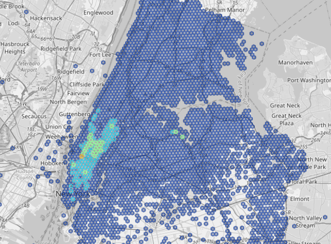
The final spatial operation I want to cover is binning and aggregation. We will use the stream of taxi trips from New York City for this section. This data contains information about the pickup and drop-off locations, fare and distance of each taxi trip in New York City. We are interested in finding hotspots in the taxi locations in the city.
Spatial binning is a technique used in data analysis to group geographically referenced data into user-defined bins or areas. The technique is used to reduce the resolution of a dataset, making it easier to visualize and analyze large datasets. This can be done by dividing the area into equal-sized rectangular grids, circles, polygons or hexagons. The resulting bins are then used for statistical analysis, such as calculating the frequency of events or measuring average values.
Kinetica offers multiple ways to generate grids for binning data: ST_HEXGRID or using H3 geohashing functions. Let’s use the latter.
Uber developed H3 (Hexagonal Hierarchical Spatial index) for efficiently optimizing ride pricing and visualizing and exploring spatial data. Each grid in the systems has an associated index and a resolution.
We can use the STXY_H3 function to identify the corresponding grid index value for each taxi drop-off and pickup location for the taxi data stream — into which hexagon a particular point falls.
Note that the materialized view is set to refresh on change, so as new data hits the system (a few hundred trips every second), the view below is automatically maintained by calculating the H3 index values for all the new records.
CREATE OR REPLACE MATERIALIZED VIEW nytaxi_h3_index
REFRESH ON CHANGE AS
SELECT
    pickup_latitude,
    pickup_longitude,
    STXY_H3(pickup_longitude, pickup_latitude, 9) AS h3_index_pickup,
    STXY_H3(dropoff_longitude, dropoff_latitude, 9) AS h3_index_dropff
FROM taxi_data_streaming;
Once we have the index values, we can use those to generate the corresponding bins using the ST_GEOMFROMH3 function. The data is then grouped by the index to calculate the total number of pickups in each bin. This is another materialized view that is listening for changes to the materialized view we set up in the query above. Again the aggregations are automatically updated and as new records arrive, the view will always reflect the most up-to-date aggregation without any additional work on our part.
CREATE OR REPLACE MATERIALIZED VIEW nytaxi_binned
REFRESH ON CHANGE AS
SELECT
    h3_index_pickup,
    ST_GEOMFROMH3(h3_index_pickup) AS h3_cell,
    COUNT(*) AS total_pickups
FROM nytaxi_h3_index
GROUP BY h3_index_pickup
The map below shows the results. We can see that the hotspots for pickup are mostly in Lower Manhattan.
Try This on Your Own
You can try all of this on your own for free using the Spatial Analytics workbook on Kinetica Cloud, or by downloading the workbook from our GitHub repo here and importing it into Kinetica’s Developer Edition. I have preconfigured all the data streams so you don’t have to do any additional set up to run this workbook.
Both Kinetica Cloud and Developer Edition are free to use. The cloud version takes only a few minutes to set up, and it is a great option for quickly touring the capabilities of Kinetica. However, it is a shared multitenant instance of Kinetica, so you might experience slightly slower performance.
The developer edition is also easy to set up and takes about 10 to 15 minutes and an installation of Docker. The developer edition is a free personal copy that runs on your computer and can handle real-time computations on high-volume data feeds.