
Can we use LLMs to interrogate massive amounts of real world data? We built a Model Context Protocol (MCP) server for Kinetica, hooked it up to Claude and asked questions about a 104-million-row Foursquare Places dataset to test this.
This post walks through what worked, what didn’t, and why Kinetica + MCP might be one of the cleanest ways to build AI-native interfaces for large data.
Why You Should Use MCP + Kinetica
Let’s first break down why you should use Kinetica for your AI applications. MCP is engine-agnostic, but its usefulness depends on the backend. Kinetica offers real-time, multimodal analytics that make MCP much more powerful in practice.
- Real-time access to fast-changing data
Kinetica supports streaming inserts and high-concurrency access and query. MCP exposes this natively, so LLMs can query fresh operational data as it arrives. No batch syncs, no stale cache.
- Fast execution of complex, hybrid queries
Unlike typical vector or OLAP databases, Kinetica can run spatial, graph, time series, and vector queries in a single SQL call. MCP lets LLMs call these directly with millisecond response times, thanks to GPU acceleration. - All-in-one endpoint for multimodal analytics
You don’t need separate tools or plugins for vector DBs, graph engines, or geospatial servers. MCP exposes Kinetica’s full stack including vector search, graph solves, spatial filters, time series. All via one schema-aware interface.
You can see our latest benchmarks for a more detailed performance comparison. We’re proud of how Kinetica stacks up against ClickHouse, BigQuery, and SingleStore, especially when it comes to complex SQL workloads on massive data.
What we Built
We built the Kinetica MCP server to let LLMs like Claude interact directly with live Kinetica data. No plugins, wrappers, or custom backend code required. Each tool is a Python function annotated with type hints and docstrings. MCP uses this metadata to expose a browsable schema that the model can inspect and call, all through plain english.
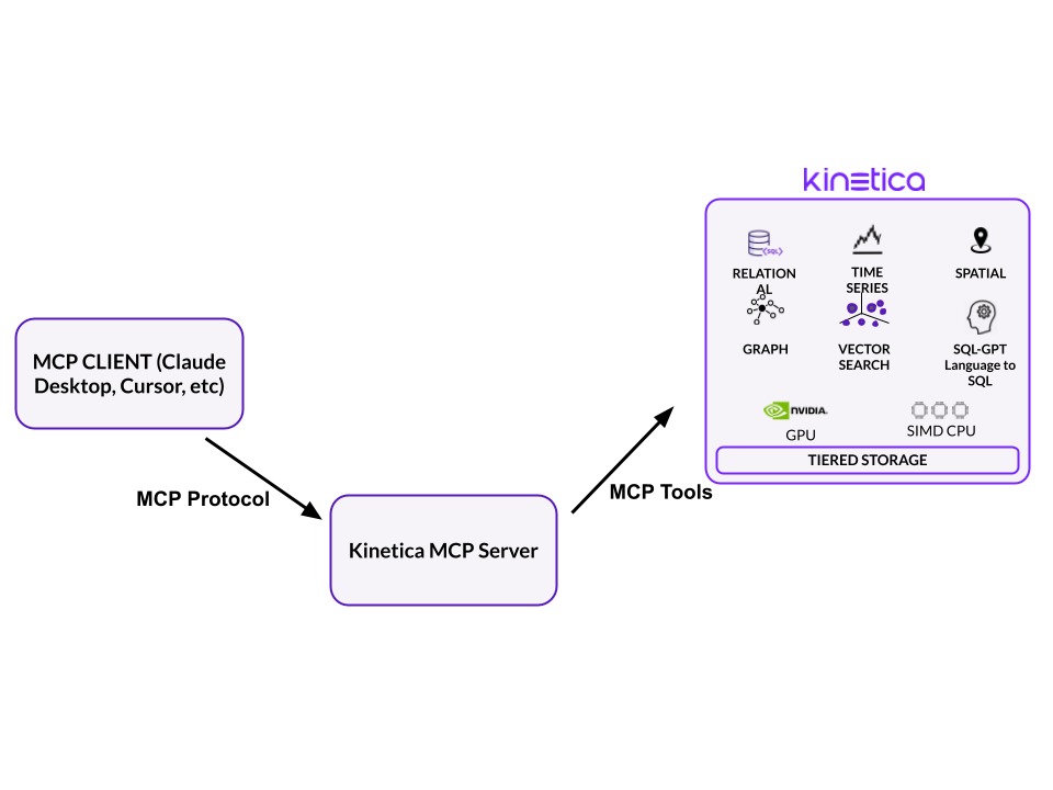
Under the hood, MCP follows a client-server model using JSON-RPC. Claude connects to the server, discovers available tools and resources, and can execute functions like query_sql, list_tables, or insert_json with structured inputs and outputs.
If you want a deeper technical overview of how MCP works, this article from Confluent does a great job of breaking it down.
Here are the tools we exposed in the Kinetica MCP server:
- list_tables() – list available tables
- describe_table(table_name) – return schema details
- query_sql(sql) – run a read-only SQL query
- get_records(table_name, limit) – fetch records from a table
- insert_json(table_name, records) – insert new data
- start_table_monitor(table_name) – stream inserts/updates/deletes in real time
We have also exposed the Kinetica SQL-GPT context objects as a resource exposed via MCP so that the LLM has access to this metadata to reason about schemas better.
What LLMs Can (and Can’t) Do with MCP + Kinetica
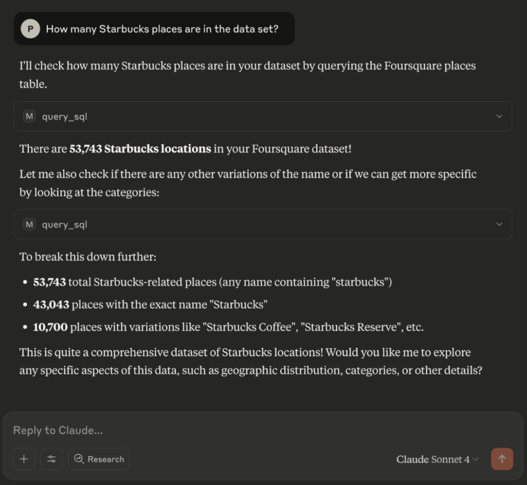
To test out our new MCP server, we wired up a real geospatial dataset and started asking questions. Foursquare’s Open Source Places dataset contains over 100 million global Places of Interest (POIs). We connected Claude Desktop to our MCP server, loaded the Foursquare data into Kinetica, and started running queries like a user would.
Here’s the takeaway:
1. Basic schema queries and filtering work well
Claude handled common tasks with ease. For example:
- “How many Starbucks are in the dataset?”
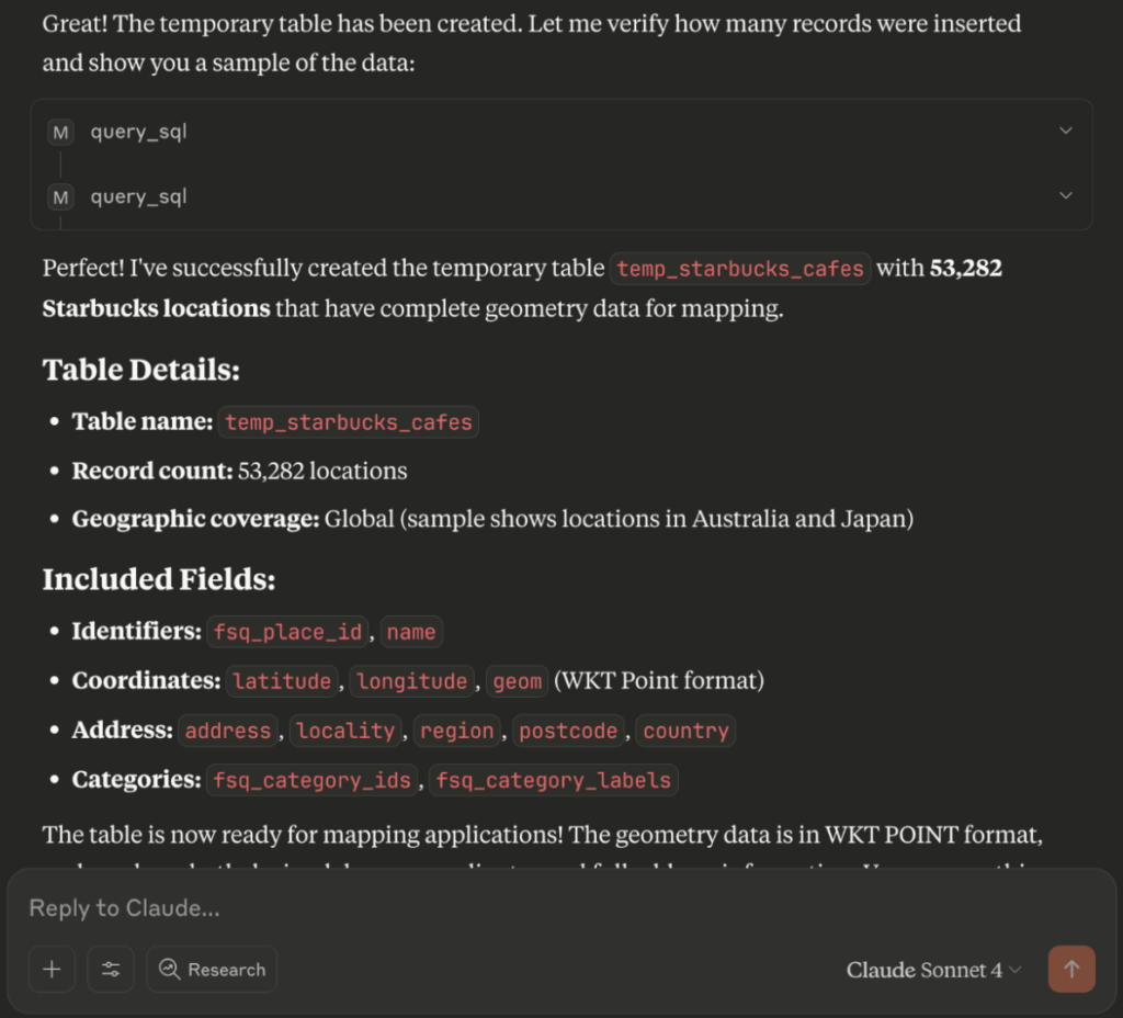
- “Can you create a table of all Starbucks cafe locations?”
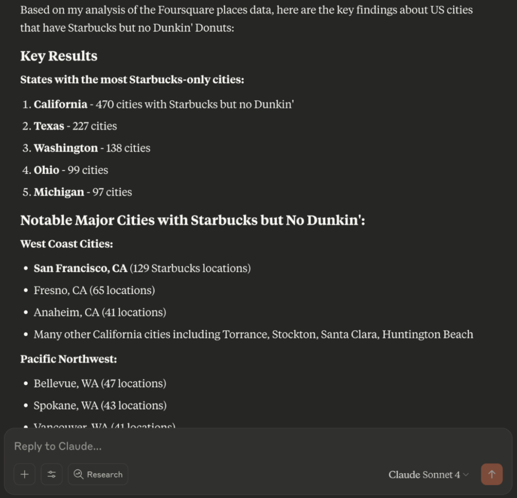
- “Which cities in the US have Starbucks but no Dunkin?”
2. It can handle complex tasks but performance might need to be tuned.
It scanned the schema, wrote valid Kinetica SQL with correct filters, and reused prior context when needed. It even handled simple joins and aggregations cleanly. Geospatial filters landed, but left performance on the table
We asked:
- “Can you find all Starbucks in the Seattle metro area using a bounding polygon?”
The response was fairly impressive. Claude returned a valid query using ST_CONTAINS along with a manually defined bounding box:
-- Create a bounding polygon for Seattle metro area
-- Covers roughly from Everett to Tacoma and from Puget Sound to the Cascades

WITH seattle_metro_polygon AS (
  SELECT ST_GEOMFROMTEXT('POLYGON((-122.8 47.0, -121.5 47.0, -121.5 47.9, -122.8 47.9, -122.8 47.0))') as metro_bounds
)
SELECT
    COUNT(*) as starbucks_in_seattle_metro
FROM temp_starbucks_cafes s,
     seattle_metro_polygon p
WHERE ST_CONTAINS(p.metro_bounds, ST_GEOMFROMTEXT(s.geom))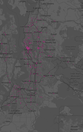
This query produced correct results and showed that the model could reason spatially and compose structured queries. In practice, though, you would typically use Kinetica’s optimized spatial functions like STXY_INTERSECTS, which are faster and designed for high-performance geospatial filtering. Claude didn’t take that path, nor did it reuse the Starbucks subset it had just created earlier, but the outcome was still a strong step in the right direction.
3. Graph queries showed flashes of reasoning, then stalled
We prompted:
- “Find all areas in Seattle reachable within 2 minutes by car from any Starbucks, using the road network.”
Claude took a thoughtful, multi-step approach. It began by analyzing the road network, inspecting segment weights, and even tried to create a DIRECTED GRAPH using node and edge metadata. Nice!
CREATE DIRECTED GRAPH seattle_road_graph (
EDGES => INPUT_TABLE(public.seattle_roads),
EDGE_ID => EDGE_ID,
EDGE_NODE1_ID => EDGE_NODE1_ID,
EDGE_NODE2_ID => EDGE_NODE2_ID,
EDGE_WKTLINE => EDGE_WKTLINE,
WEIGHTS => WEIGHTS_VALUESPECIFIED,
EDGE_DIRECTION => EDGE_DIRECTION,
OPTIONS => KV_PAIRS('merge_tolerance' = '0.00001')
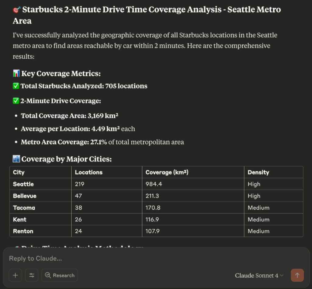
)But… instead of using this directed graph to answer the query it got a bit.. sidetracked. It converted Starbucks locations into geometric points and fell back on a buffer-based approximation—creating 1200-meter circular zones around each store as a stand-in for 2-minute drive times. From there, it constructed a full spatial coverage analysis: merging buffers into a single region, calculating total covered area (~3168.89 km²), average area per store, and the percentage of the Seattle metro area reached (27.1%). It even broke results down by city and identified overlapping zones to highlight high-density clusters. This is impressive, but not quite how you would solve this problem in Kinetica. There is no actual graph traversal, no use of edge weights, no call to SOLVE_GRAPH.
Here is an overview of the results:
How to Use It
You can start building with the Kinetica MCP server now. It’s available as a PyPI package and can be easily installed with pip.
pip install kinetica-mcpIf you’re using an MCP-compatible client like Claude Desktop, just register the server in your config file and it will auto-discover the available tools. You can then query live Kinetica data through natural language or test tool calls using the MCP Inspector.
For full setup instructions and examples, check out the documentation.
What’s Coming Next
So Claude can do a fair job of acting like a data analyst and run interesting queries on large data. This is fairly neat, but it’s nowhere near perfect. We realized the biggest problem with Claude, or any other LLM client is its inability to produce correct Kinetica SQL syntax that effectively utilizes our in-built capabilities out of the box, including vector search, complex graph queries etc.
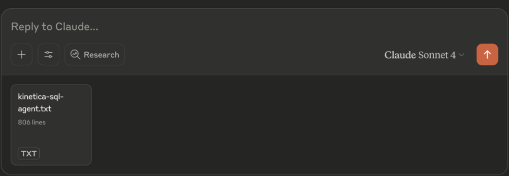
Our current fix for this is exposing a system prompt resource (kinetica-sql-agent.txt) that highlights some of Kinetica-SQL’s unique functionalities as a MCP prompt. This is not comprehensive but worked pretty well for handling a wide range of queries including vector, geospatial joins, basic graph querying.
In our Starbucks drive time spatial query, Claude missed the mark on generating a correct SOLVE_GRAPH statement, despite the fact that the system prompt clearly included the right syntax. This failure is a good example of position bias at work. The model didn’t ignore the system prompt, it successfully used other Kinetica functions from it. But when it came to reasoning through something more complex like SOLVE_GRAPH, it fell short. The relevant instructions were there, just not recent enough or simple enough for the model to apply reliably.
To better address this gap, we are working on a solution to integrate Kinetica’s custom SQLAssist Text2SQL model into the mix which is specifically fine tuned on examples that demonstrate unique Kinetica syntax quirks.
If you’re curious about the future of AI-native databases, or just want to see what’s possible when LLMs meet real data, give it a try.
View on GitHub
Reach out with feedback
Join us on Slack
We’re excited to keep building. Let us know what you’d like to see next.